Introduction
The LLL Reduction Algorithm is a Lattice Basis Reduction technique. It transforms a given basis of a lattice into one with short, nearly orthogonal vectors. The LLL Reduction Algorithm uses the Gram-Schmidt Algorithm in order to find a short, orthogonal basis.
In order to understand the LLL Reduction Algorithm, we must first understand how the Gram-Schmidt Algorithm finds a basis that has the same span as the original basis.
What does it mean to reduce a lattice?
A lattice is composed of all possible integer combinations of its basis vectors. Imagine that we have 2 linearly independent vectors, \(v_1\) and \(v_2\). The lattice would be defined as \(L = \{av_1 + bv_2:\forall a, b \in \mathbb{Z}\}\). It can be proven that a lattice has an infinite amount of possible basis vectors that can construct it. Most of the time the basis vectors of our lattice is ugly, for example 2 basis vectors that are almost parallel. This makes it hard for them to work with, instead we can perform a lattice reduction onto these 2 almost parallel vectors, into 2 shorter and orthogonal vectors.
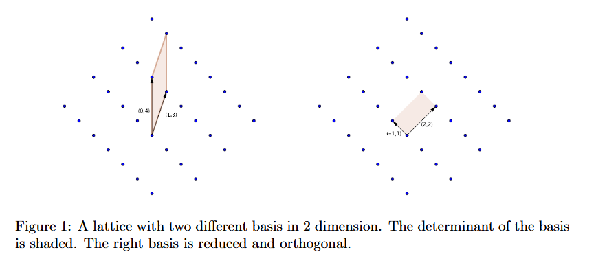
SVP solved for 2D Lattice by Gauss
Gauss solve SVP for 2D lattices through a clever trick that even you might have used in physics. As we are working in 2 dimensions, we will only be working with 2 basis vectors, let our basis vectors be \(B = \{b_1, b_2\}\)
If \(\vert\vert b_1 \vert\vert > \vert\vert b_2 \vert\vert\) swap the vectors \(b_1\) and \(b_2\). Then we calculate the projection coefficient of \(b_2\) onto \(b_1\) (We will cover what projection coefficient is later) which is given by this formula \(\mu = \frac{b_1 \cdot b_2}{\vert\vert b_1 \vert\vert ^ 2}\). If \(\mu > \frac{1}{2}\), then we let \(m\) be the nearest integer of \(\mu\). We then reassign \(b_2 = b_2 - mb_1\). If \(\vert\vert b_1 \vert\vert > \vert\vert b_2 \vert\vert\), swap \(b_1\) and \(b_2\) and run the full algorithm again. When it finally finishes we would have obtained a set of basis vectors that cover the exact same lattice, however, they are the shortest possible vectors and are also orthogonal. (Meaning that they are perpendicular)
Intuitively, what this means is that we take the longer vector, and see how many smaller vectors it contains and take that away, as it is an integer combination of 2 vectors, that vector is still valid on the same lattice. We perform this algorithm until we are unable to reduce the size of both vectors.
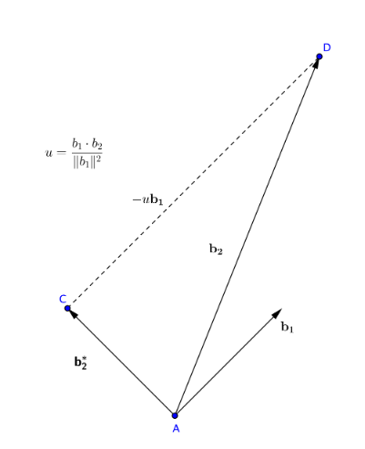
Projection + Projection Coefficient
Projection is simply telling you how much a vector contains another vector. An analogy that I can make is through physics. In projectile motion, we have an object with a velocity, \(v\). In order to make calculations easier, we often split up this velocity into \(v_x\) and \(v_y\) where they are the x-component and y-component of the initial velocity. A projecrtion is similar in idea, however, instead of having some predetermined vector like \(v_x\) or \(v_y\), we simply use another vector of our choice. After calculating the projection of a vector, \(v_1\), on another vector, \(v_2\), we will get a resulting vectors in the form of \(\mu v_2\) where \(v_1 = v_1^* + \mu v_2\) where \(\mu\) is the projection coefficient.
Formulas:
\[\mu u = \text{proj}_u (v) = \frac{\langle v, u \rangle}{\langle u, u\rangle} \cdot u\] \[\mu_{i, j} = \frac{\langle \vec{v_i}, \vec{u_j}\rangle}{\langle \vec{u_j}, \vec{u_j}\rangle}, j < i\]Gram Schmidt Algorithm
The Gram Schmidt Algorithm is the core part of the LLL Reduction Algorithm and looks very similar to Gauss’ Algorithm for solving SVP in 2D. However, it is unable to solve the SVP for Lattices, but it can solve SVP for span using linear combinations of the initial vectors.
The Gram Schmidt Algorithm first starts off by letting the first original basis vectors be the first new basis vectors, the algorithm will then make every other vector orthogonal to thi first new basis vector.
\[u_1 = v_1\] \[u_2 = v_2 - \text{proj}_{u_1} (v_2)\] \[u_3 = v_3 - \text{proj}_{u_1} (v_3) - \text{proj}_{u_2} (v_3)\] \[\dots\] \[u_k = v_k \sum_{j = 1}^{k - 1} \text{proj}_{u_j} (v_k)\]The algorithm simply returns \((u_1, \dots, u_k)\) which is a tuple of basis vectors that are orthogonal to each other, that also have a linear relationship with the original set of vectors.
Size Reduction Condition
The size reduction condition is given by:
\[\vert \mu_{i, j} \vert \leq \frac{1}{2}\]When the projection coefficient is larger than \(\frac{1}{2}\), we know that we can subtract an integer amoutn fo the vector beign projected on in order to further reduce the size of the basis vectorzs. This operation is done on the original vectors.
\[v_i \leftarrow v_i - \lfloor \mu_{i, j} \rceil v_j\]Lovasz Condition
Lovasz Condition is a condition that locally optimises/greed the shortness of the basis vectors. It does this by running the full algorithm and seeing if swapping the order in which the vectors are inputted into the Gram Schmidt Algorithm would result in shorter orthogonal vectors. There are methods in order to solve ofr exact SVP for n dimensions, however, they are not in polynomial time. Lovasz Condition allows for optimisation while allowing LLL to remain in polynomial time.
The Lovasz Condition is given by:
\[\delta \vert\vert u_{k - 1} \vert\vert ^2 \leq \vert\vert u_k \vert\vert ^2 + \mu^2_{k, k - 1}\vert\vert u_{k - 1} \vert\vert ^2\]where \(\delta\) usually equals \(\frac{3}{4}\). Delta represrents the degree of reduction, where the greater \(\delta\) is, the more reduced the resultant vector will be. However, the polynomial time complexity is only guaranteed where \(\delta \in (0.25, 1)\)
If the conditions is not fulfilled, the order of the vectors outputted from the Gram Schmidt Algorithm is swapped.
LLL Reduction Algorithm
The LLL Reduction Algorithm starts off by inputting the “messy” vectors \((v_1, \dots, v_k)\) into the Gram Schmidt Algorithm, this outputs us a set of new vectors \((u_1, \dots, u_k)\). These new vectorrs can be composed by a linear equation formed by the messy set of vector, however, their coefficients may not be integers. (This means that they do not cover the same lattice, we will fix this later). In order for this new set of vectors to fulfil the original set of lattices, we need to round the projection coefficient to integer values. This will make out vectors nearly orthogonal instead of completely orthogonal.
We will then continue to further optimize the length of our vectors by applying the Size Reduction Condition and Lovasz Condition to our projection coefficients and Gram Schmidt reduced vectors. After every condition has been satisfied, we have obtained our new set of short and nearly orthogonal set of basis vectors that fulfill the same lattice as the original set of vectors.
Significance + Demo
The LLL Algorithm has many applications, and one of its many application is in cryptography. The LLL Algorithm is used to break down certain vulnerabilities in RSA and ECDSA. It can also be used to find rational solutison to Linear Diophantine Equations, ehre is a demonstration of how we do it. Let’s say that we are given this equation: \(ax_1 + bx_2 + cx_3 = d\), where \(a, b, c, d\) are known and \(x_1, x_2, x_3\) are our integer unknowns. In order to solve it, we must express our unknowns as the solution to a known set of basis vectors. We use a clever method where we use dummy 1s and 0s in order to construct such an equation.
\[\begin{pmatrix} a \\ 1 \\ 0 \\ 0 \end{pmatrix}x_1 + \begin{pmatrix} b \\ 0 \\ 1 \\ 0 \end{pmatrix}x_2 + \begin{pmatrix} c \\ 0 \\ 0 \\ 1 \end{pmatrix}x_3 - \begin{pmatrix} -d \\ 0 \\ 0 \\ 0 \end{pmatrix} = \begin{pmatrix} 0 \\ x_1 \\ x_2 \\ x_3 \end{pmatrix}\]This gives us a set of basis vectors that we can put into a matrix and perform LLL on it, allowing us to derive an integer solution for our unknowns. Thank you for reading!